How this blog works

Sidenotes, margin notes, and LaTeX, with the sliced Wasserstein distance as a running example

September 25, 2026

I have discovered a truly marvelous proof of this, which this margin is too narrow to contain.
Pierre de Fermat, note in his copy of Diophantus’s Arithmetica, c. 1637

Every post here is a Markdown file in content/blog/. The layout follows Edward Tufte’s books: a narrow main column, with notes living beside the text instead of at the bottom of the page.On a phone the notes fold away; tap the superscript number to open one. This post uses each feature once, so it doubles as a reference. Delete it, or set draft: true in its front matter, once the first real post is up.

Mathematics

Write LaTeX exactly as you would in a paper. Inline math goes between single dollar signs and display math between double dollar signs, or in any standard environment. Underscores and backslashes are handed straight to MathJax, so Markdown never mangles them.

For probability measures $\mu,\nu$ on $\R^d$ with finite $p$th moments, the $p$-Wasserstein distance is

\begin{equation}\label{eq:wp} W_p(\mu,\nu) = \Big( \inf_{\pi \in \Pi(\mu,\nu)} \int \norm{x-y}^p \, d\pi(x,y) \Big)^{1/p}, \end{equation}

where $\Pi(\mu,\nu)$ is the set of couplings of $\mu$ and $\nu$. In one dimension it has a closed form,If $F_\mu^{-1}$ and $F_\nu^{-1}$ are the quantile functions, then $W_p^p(\mu,\nu) = \int_0^1 \abs{F_\mu^{-1}(t) - F_\nu^{-1}(t)}^p \, dt$, because the monotone coupling is optimal for convex costs on the line. which is what makes projecting attractive. For $\theta$ on the unit sphere $S^{d-1}$, write $\theta_\#\mu$ for the law of $\ip{\theta}{X}$ when $X \sim \mu$. Then

\begin{align} \mathrm{SW}_p(\mu,\nu) &= \Big( \int_{S^{d-1}} W_p^p(\theta_\#\mu, \theta_\#\nu) \, d\sigma(\theta) \Big)^{1/p}, \label{eq:sw} \\ \overline{W}_p(\mu,\nu) &= \max_{\theta \in S^{d-1}} W_p(\theta_\#\mu, \theta_\#\nu), \label{eq:msw} \end{align}

where $\sigma$ is the uniform probability measure on the sphere.

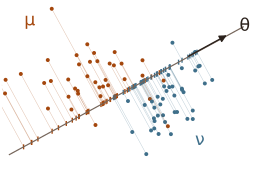⊕ Two point clouds in the plane, each point joined to its projection on a line through the origin Two samples in $\R^2$ and their projections onto a direction $\theta$. Each projection is a one-dimensional transport problem.Equations are numbered automatically and can be cited with \eqref. Since $x \mapsto \ip{\theta}{x}$ is 1-Lipschitz, pushing an optimal coupling in \eqref{eq:wp} forward through it shows $W_p(\theta_\#\mu,\theta_\#\nu) \le W_p(\mu,\nu)$ for every $\theta$. Averaging over $\theta$ in \eqref{eq:sw}, and maximizing in \eqref{eq:msw}, then gives

\mathrm{SW}_p(\mu,\nu) \;\le\; \overline{W}_p(\mu,\nu) \;\le\; W_p(\mu,\nu).

Reverse inequalities are much subtler.⊕This is a margin note: like a sidenote, but without a number.

Code

Fenced code blocks are highlighted. Here is a Monte Carlo estimate of \eqref{eq:sw} for two samples of the same size, using the fact that on the line the optimal coupling matches sorted points:

import numpy as np

def sliced_wasserstein(X, Y, n_proj=500, p=2, seed=0):
    """Monte Carlo estimate of SW_p between two equal-size samples."""
    rng = np.random.default_rng(seed)
    theta = rng.standard_normal((n_proj, X.shape[1]))
    theta /= np.linalg.norm(theta, axis=1, keepdims=True)
    x_proj = np.sort(X @ theta.T, axis=0)
    y_proj = np.sort(Y @ theta.T, axis=0)
    return np.mean(np.abs(x_proj - y_proj) ** p) ** (1 / p)

Quick reference

To get	Write
Numbered sidenote	`{{< sidenote >}}…{{< /sidenote >}}`
Unnumbered margin note	`{{< marginnote >}}…{{< /marginnote >}}`
Small-caps opening	`{{< newthought >}}…{{< /newthought >}}`
Figure in the margin	`{{< marginfigure src="plot.svg" caption="…" >}}`
Figure, caption in margin	`{{< figure src="plot.png" caption="…" >}}`
Opening quotation	`{{< epigraph author="…" >}}…{{< /epigraph >}}`
A literal dollar sign	`\$`

Shortcuts such as \R, \E{X}, \norm{x}, and \ip{x}{y} are defined in assets/macros.tex, written just as in a LaTeX preamble; add your own there.